


Continuous time dimensions and persistence
Davide Faranda computed the local dimension d and local persistence θ of the daily SLP field from the NCEP reanalysis (Faranda et al., Sci. Rep. 2017).
The local dimension and persistence are compared to the weather regime classification.
a) The scatter plot displays the daily values of the instantaneous dimension d – the higher d, the more unpredictable is the atmospheric circulation – and the persistence θ – the lower θ the more stable is the atmospheric circulation – of the sea level pressure field (in hPa) extracted from the NCEP Database and the forecast up to 72h extracted from the GFS model. The trajectory for the last 7 days is displayed in colors. b) The weather regimes are computed as the days beyond the 0.15 quantiles of the d and θ distribution displayed in panel a). c) Distribution of the best 25 analogues per decades. d) Percentage of days of the same month in all the database with higher or lower dimensions d . e) Same as d) but for the persistence θ. See here for explanations. f) Sea-level pressure fields over the North-Atlantic showing the domain of the analysis and forecasts +24h, 48h, 72h.
The (d,θ) variables are available here. The file is provided ‘as is’.
References
Continuous time weather regimes
Weather regimes are prefered atmospheric states (Legras and Ghil 1985; Vautard 1990). They can be computed on pressure fields with classification algorithms. We use a kmeans algorithm on sea-level pressure to determine four weather regimes over the North Atlantic region, from the NCEP reanalysis.
We use a method developed by Yiou et al. (2008) to stabilize the computation of the classes, by Monte-Carlo experiments and a classification of the experiments.
Weather regimes are computed for the four seasons (DJF, MAM, JJA and SON) on a reference period between 1970 and 2010. The whole SLP field is then classified on those reference weather regimes. Simple diagnostics are shown, with the occurrence of weather regimes in the current (or last) season, and the frequency of the weather regimes since 1948.
DJF Weather regimes
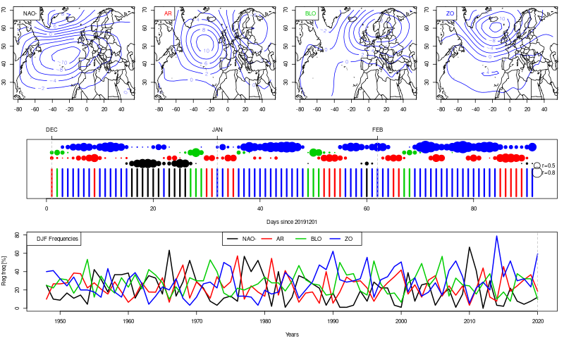
Upper panel: DJF weather regimes from NCEP SLP (reference period 1970-2010). The isolines are SLP anomalies for each centroid.
- Regime 1 is NAO-,
- Regime 2 is Atlantic RIDGE,
- Regime 3 is SCANDINAVIAN BLOCKING,
- Regime 4 is ZONAL (or NAO+).
Middle panel: daily classification since the first day of the running (or last) winter season (vertical bars). The classification is done by minimizing the rms between the observed anomaly and the weather regimes in the upper panel. The diameter of circles indicate the spatial correlation with the four weather regimes (only positive correlations are shown). Note that minimizing an rms is not equivalent to maximizing the correlation.
Lower panel: statistics of frequencies (percentage of occurrences during the season) for the four regimes since 1948. A png file can be obtained by clicking on the figure.
The complete classification file is available here. The files are updated every mondays.
MAM Weather regimes
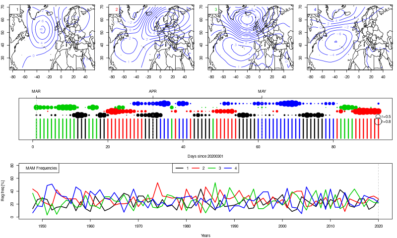
MAM frequency of weather regime and daily classification. The first line recalls the weather regimes. The second line is the daily classification since the first day of the running season. The last line is the statistics of frequencies for the four regimes.
WARNING: weather regimes of intermediate seasons (SON or MAM) are not well defined. This figure is given as an indication. Such results should not be used for research or applications.
JJA Weather regimes
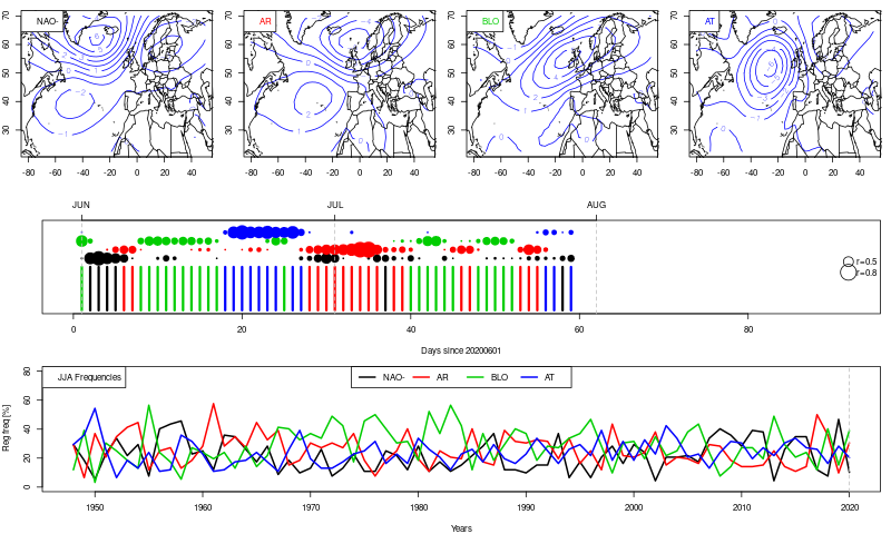
JJA frequency of weather regime and daily classification. The first line recalls the weather regimes. The second line is the daily classification since the first day of the running season. The last line is the statistics of frequencies for the four regimes.
Upper panel: JJA weather regimes from NCEP SLP (1970-2000). The isolines are SLP anomalies for each centroid.
- Regime 1 is NAO-,
- Regime 2 is Atlantic RIDGE,
- Regime 3 is SCANDINAVIAN BLOCKING,
- Regime 4 is Atlantic Thalweg (or NAO+).
Beware that the classifiability of JJA months is rather low.
Middle panel: daily classification since the first day of the running (or last) summer season. The diameter of circles indicate the spatial correlation with the four weather regimes (only positive correlations are shown).
Lower panel: statistics of frequencies (percentage of occurrences during the season) for the four regimes since 1948. A png file can be obtained by clicking on the figure.
SON weather regimes
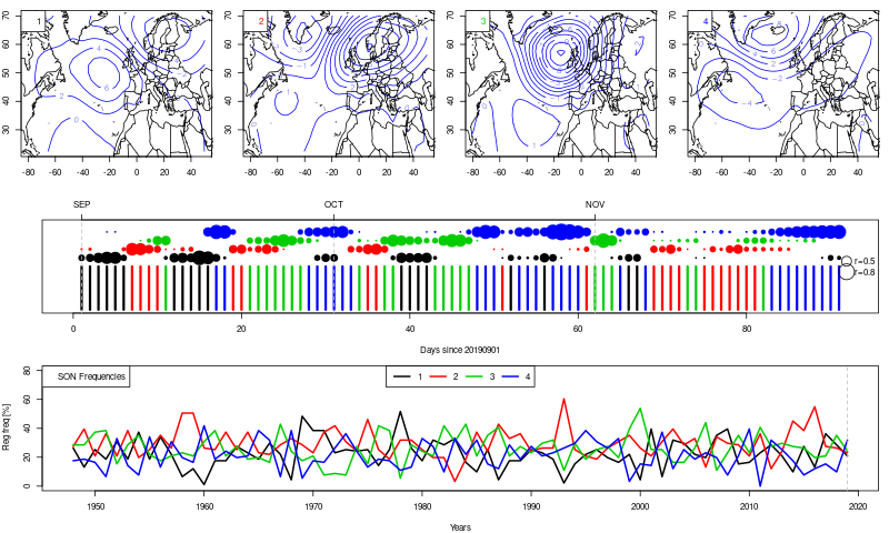
SON frequency of weather regime and daily classification. The first line recalls the weather regimes. The second line is the daily classification since the first day of the running season. The last line is the statistics of frequencies for the four regimes.
WARNING: weather regimes of intermediate seasons (SON or MAM) are not well defined. This figure is given as an indication. Such results should not be used for research or applications.
The results are updated weekly. The files for the four seasons can be found at:
http://dods.lsce.ipsl.fr/dase/REGIMES/
The pdf files show the weather regimes for each season (DJF, MAM, JJA, SON: see figure above for DJF). The dat files are the classifications of all days. The first column is the day (in yyyymmdd format). The second column is the weather regime number (identified in the corresponding figure). The third column is the distance to the weather regime.
You can use those files for your own research. They are updated every week. Please cite:
References
Legras, B. & Ghil, M. Persistent anomalies, blocking and variations in atmospheric predictability, J. Atmos. Sci., 1985, 42, 433-471
Vautard, R. Multiple weather regimes over the North Atlantic: Analysis of precursors and successors, Mon. Wea. Rev., 1990, 118, 2056-2081
Analogue Software
The A2C2 project develops open source software for the computation of atmospheric analogues. At present, the software is in a “developer” mode, i.e., it only contains a core for the computation & file manipulation. There is no cool front end with guis, graphics and those kinds of gizmos… which are under development.
R codes
The programme is a suite of scripts in shell script (sh) with ncks/nco and cdo commands, and an R script. The programme downloads and concatenates NCEP reanalysis SLP for the North Atlantic region, then computes the analogues for various distance/metrics (rms, correlations…). It runs on linux or macosX computers. It is more comfortable to have a powerful multicore computer to do the job.
By default, the analogues are computed by minimizing an rms (or Euclidean) distance. 20 “best” analogues are computed for each day between 1st Jan. 1948 and the current day. The analogues are taken from a different year than the “target” day, and are separated by at most 30 calendar days.
The R code can run in parallel on multicore computers (with the “parallel” package). It has been tested on our computing cluster with n=12 processors.
The programme is provided as is. It is free for academic use. Please contact Pascal Yiou for a commercial use. The suite of programmes is available here.
Please cite:
Yiou, P., T. Salameh, P. Drobinski, L. Menut, R. Vautard, and M. Vrac, 2013 : Ensemble reconstruction of the atmospheric column from surface pressure using analogues. Clim. Dyn., 41, 1419-1437. [.pdf]
Flyingpidgeon
A web processing service (WPS) that allows you to compute analogues, weather regimes, and much more, on reanalyses or model simulations has been developed for the A2C2 project. This WPS is called flyingpidgeon. It is compatible with a wider ecosystem of WPS (the birdhouse).
We also developed an analogue viewer, for a quick visualisation of the computation of analogues. Its experimental form can be obtained at:
http://birdhouse.readthedocs.io/en/latest/
Web Processing Service “blackswan”
The analogues can also be computed “online” from the “blackswan” WPS that is available on github.
Deliverables and products
Ensemble forecast simulations with analogues
Continuous time analogues
Analogues of atmospheric circulation are weekly computed from the SLP of NCEP (daily) reanalysis. We consider the North Atlantic region (80W-30E; 30-70N).
The evaluation of the SLP analogues is updated regularly.
Evaluation of analogues
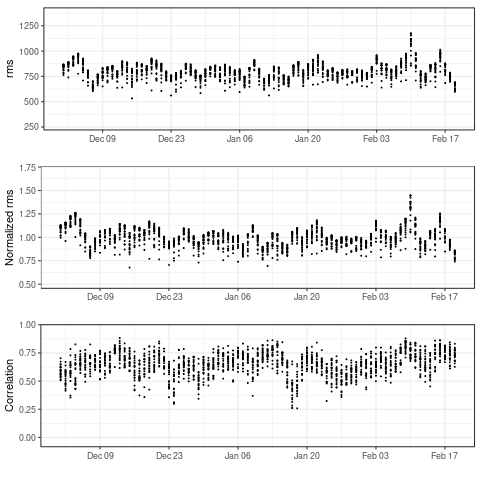
Return periods
The distribution of analogues allow to compute the probability of observing an SLP pattern (given a history of pattern) and return times of SLP patterns (the time to wait for a pattern to recur).
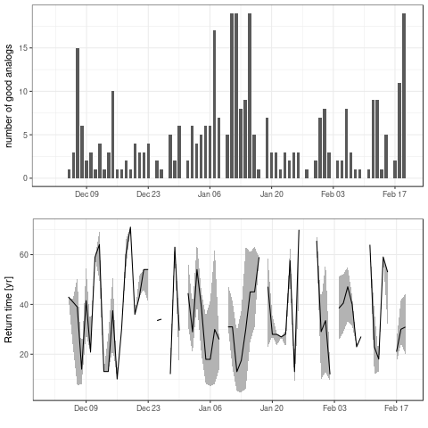
Analogue files
The analogue file contains 61 columns:
- The first column is the analyzed days (from 1st January 1948 to the current day).
- The next 20 columns are the dates of the best analogues, i.e. those that minimize an rms function. The next 20 columns are the values of the rms (actually -rms).
- The last 20 columns are the values of the spatial correlation.
It can be used as input to the Analogue Weather Generator (AnaWEGE) designed by P. Yiou (2014). The software to produce this file (including downloading NCEP reanalysis data) can be obtained from this web site.
We use this file to analyze extreme events. See for example the BAMS report on extremes.
The file is free for academic use (and is provided “as is”). Please contact Pascal Yiou for commercial uses.

